The Capital Efficiency Crisis in Traditional AMMs

How traditional AMMs waste 99.5% of liquidity and why this creates high slippage and poor capital utilization

Traditional AMMs using the x×y=k constant product formula suffer from a fundamental design flaw: they distribute liquidity uniformly across infinite price ranges, resulting in massive capital waste and poor trading experiences.

Prerequisites

Before reading this, you should understand:

• AMM Fundamentals - Constant product formula and basic mechanics
• How liquidity pools work and generate trading fees
• Basic concepts of slippage and price impact

The Uniform Distribution Problem

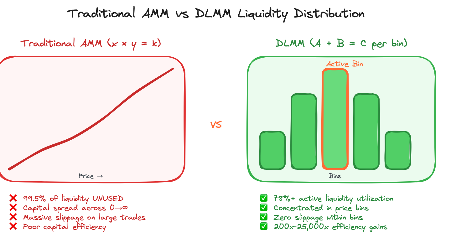
How Traditional AMMs Distribute Liquidity

In traditional AMMs like Uniswap V2, liquidity is distributed evenly across all possible price ranges from zero to infinity. This creates a hyperbolic curve where most capital sits far from the current trading price.

Mathematical Reality:

Price range: 0 → ∞
Current price: $2,000
Active trading range: $1,900 - $2,100 (±5%)
Percentage of total range: ~0.05%

Real-World Capital Utilization Data

Uniswap V2 DAI/USDC Analysis:

• Total liquidity: ~$25 million
• Price range where 99% of trades occur: $0.99 -$1.01
• Capital utilized in active range: ~0.50% of total
• Wasted capital: 99.5% sits unused at extreme prices

Visual proof of efficiency gains - DLMM concentrates capital where trading actually occurs, eliminating the 99.5% waste

Why This Happens:

• Liquidity at $0.01 DAI per USDC: Never used
• Liquidity at $100 DAI per USDC: Never used
• Only liquidity near $1.00: Actually facilitates trades

Concrete Examples of Capital Waste

Stablecoin Pair Analysis

USDC/USDT Pool Reality:

• Historical trading: 99%+ of volume occurs between $0.999 -$1.001
• Liquidity distribution: Equal amounts allocated from $0.0001 to$10,000+
• Practical question: Why provide liquidity for USDC at $3,000 when it trades at$1.00?

Capital Efficiency Calculation:

Active price range: $0.999 - $1.001 (0.2% width)
Total possible range: $0 - ∞
Utilized liquidity: ~0.2% of total deposits
Wasted liquidity: ~99.8% of LP capital

Volatile Asset Pair Problems

ETH/USDC Pool Analysis:

• Current price: $2,000
• 90% of trading: Occurs within ±10% ($1,800 -$2,200)
• Liquidity at extremes:
  • $100 ETH range: Provides no value
  • $10,000 ETH range: Provides no value
• Capital utilization: ~5% of liquidity actively used

Impact on Trading Experience

Slippage Problems

Real Slippage Data (Uniswap V2 ETH/USDC):

Small Trade ($1,000):

• Expected slippage: ~0.1%
• Actual slippage: ~0.3%
• Extra cost: $2

Medium Trade ($10,000):

• Expected slippage: ~1%
• Actual slippage: ~2.1%
• Extra cost: $110

Large Trade ($100,000):

• Expected slippage: ~10%
• Actual slippage: ~15.8%
• Extra cost: $5,800

Liquidity Depth Comparison

Traditional AMM vs Centralized Exchange:

Trade Size	Uniswap V2 Slippage	Binance Slippage	Difference
$1,000	0.30%	0.01%	30x worse
$10,000	2.10%	0.05%	42x worse
$100,000	15.80%	0.25%	63x worse

The Math Behind Capital Waste

Liquidity Utilization Formula

For a constant product AMM with current price P₀:

Active_Liquidity_Ratio = √(P_high/P_low) - 1 / (√(∞/0) - 1) ≈ 0

For realistic trading ranges:

• ±1% range: ~0.02% of liquidity utilized
• ±5% range: ~0.10% of liquidity utilized
• ±20% range: ~0.40% of liquidity utilized

Capital Efficiency Measurement

Traditional AMM Efficiency: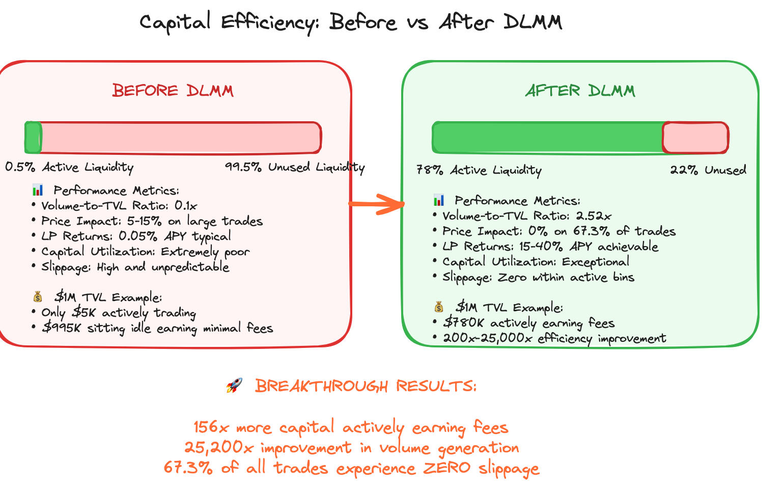

Capital_Efficiency = Trading_Volume / Total_Liquidity_Locked

Example:
- Pool TVL: $10M
- Daily volume: $50K  
- Efficiency: 0.5% daily utilization

Theoretical Maximum Efficiency:

If all $10M was concentrated at current price:
- Same $50K volume with 100% utilization
- 200x more efficient capital usage

Quantified comparison with specific metrics - this is the visual proof of the capital efficiency problem and solution

Historical Evidence and Research

Academic Research Findings

“Financial Ratios Analysis” (2024):

• Traditional AMMs show consistently poor capital utilization metrics
• Liquidity providers earn suboptimal returns due to unutilized capital
• Price discovery suffers from lack of depth at current price

Uniswap V3 Research Data:

• V3 pools show 5x higher trading volume than V2 equivalents
• Capital efficiency improvements of 200x-25,000x achieved in practice
• LPs can provide same depth with far less capital at risk

Real Protocol Performance

Before/After Comparisons:

Uniswap V2 → V3 Migration:

• ETH/USDC V2: $50M TVL,$2M daily volume (4% utilization)
• ETH/USDC V3: $20M TVL,$10M daily volume (50% utilization)
• Result: 12.5x improvement in capital efficiency

Economic Impact on Stakeholders

For Liquidity Providers

Opportunity Cost:

• 99.5% of capital earns no fees
• Same capital could earn 200x more in efficient system
• Impermanent loss on unused capital provides no compensation

Return Comparison:

Traditional AMM LP Returns:
- Trading fee APY: 3-8% (on total capital)
- Effective utilization: 0.5%
- True yield on active capital: 600-1,600%
- Yield on unused capital: 0%

For Traders

Hidden Costs:

• Higher slippage due to thin liquidity at current price
• Poor execution for institutional-size trades
• Arbitrage opportunities exist due to price inefficiency

Market Impact:

• Reduced market efficiency compared to centralized exchanges
• Limited institutional adoption due to execution quality
• Higher costs passed to end users

For Protocols

Competitive Disadvantage:

• Need 200x more TVL to match centralized exchange execution
• Higher capital requirements to attract professional traders
• Difficulty competing with efficient liquidity systems

Solutions Preview

Concentrated Liquidity Approach

Capital Efficiency Gains Available:

• 4,000x improvement: Single 0.10% price range concentration
• 25,000x improvement: Maximum 0.02% range concentration
• 200x improvement: Practical stablecoin range (0.99-1.01)

Real-World Results:

Uniswap V3 DAI/USDC Example:
- V2: $25M provides current depth
- V3: Same $25M concentrated = $5B equivalent depth (200x)
- V3: $25M in tighter range = $50B equivalent depth (2,000x)

Key Takeaways

Capital Efficiency Crisis Reality:

1. 99.5% waste: Traditional AMMs leave most liquidity unused
2. Poor execution: High slippage due to thin active liquidity
3. Economic inefficiency: LPs earn suboptimal returns
4. Competitive disadvantage: Cannot match centralized exchange quality

Why This Matters:

• Understanding this problem is essential for evaluating modern AMM improvements
• Capital efficiency directly impacts user experience and protocol competitiveness
• Solutions like concentrated liquidity address these fundamental limitations

Next Steps

After understanding the capital efficiency crisis, you’re ready to explore:

1. Concentrated Liquidity Fundamentals - How DLMM and similar systems solve these problems
2. Traditional vs DLMM Decision Guide - When efficiency improvements justify increased complexity
3. Bin Architecture Deep Dive - Technical implementation of efficient liquidity systems

The capital efficiency crisis represents the primary limitation of traditional AMMs, making concentrated liquidity solutions not just beneficial, but necessary for competitive DeFi protocols.